2 Data

Code

library(dplyr)
library(tidyverse)
library(readxl)
library(tidyquant)
library(glue)
library(tidyr)
library(lubridate)

2.1 Description

Interest rate data from 2022-2023 Daily interest rate data is collected by U.S Department of the Treasury and is downloaded as csv files. The data consists of 1 month rates to 30 year rates and is updated daily, note that since 10/18/2022 there are no 4 months interest rates.

Code

APR21 = read.csv("daily-treasury-rates-2021.csv")
APR22 = read.csv("daily-treasury-rates-2022.csv")
APR23 = read.csv("daily-treasury-rates-2023.csv")
APR = bind_rows(APR21,APR22,APR23)
head(APR)

        Date X1.Mo X2.Mo X3.Mo X6.Mo X1.Yr X2.Yr X3.Yr X5.Yr X7.Yr X10.Yr
1 12/31/2021  0.06  0.05  0.06  0.19  0.39  0.73  0.97  1.26  1.44   1.52
2 12/30/2021  0.06  0.06  0.05  0.19  0.38  0.73  0.98  1.27  1.44   1.52
3 12/29/2021  0.01  0.02  0.05  0.19  0.38  0.75  0.99  1.29  1.47   1.55
4 12/28/2021  0.03  0.04  0.06  0.20  0.39  0.74  0.99  1.27  1.41   1.49
5 12/27/2021  0.04  0.05  0.06  0.21  0.33  0.76  0.98  1.26  1.41   1.48
6 12/23/2021  0.04  0.05  0.07  0.18  0.31  0.71  0.97  1.25  1.42   1.50
  X20.Yr X30.Yr X4.Mo
1   1.94   1.90    NA
2   1.97   1.93    NA
3   2.00   1.96    NA
4   1.94   1.90    NA
5   1.92   1.88    NA
6   1.94   1.91    NA

Downloaded sp500 portfolio from https://www.slickcharts.com/sp500 as sp500rank.xlsx

Code

sp500rank <- read_excel("sp500rank.xlsx")
sp500rank_list = unlist(sp500rank['Symbol'])
top_105_symbols = sp500rank_list[1:105]
last_105_symbols = rev(rev(sp500rank_list)[1:105])

The stock symbols are then used to download 20 year daily movement from yahoo finance

Code

options("getSymbols.warning4.0"=FALSE)
options("getSymbols.yahoo.warning"=FALSE)
#getSymbols(top_105_symbols, from = '2003-10-30', to = "2023-10-30",warnings = FALSE)
#for (symbol in top_105_symbols) {
#  if (exists(symbol)) {
#    write.zoo(get(symbol), glue('data/{symbol}.csv'), sep = ",")
#  }
#}
#getSymbols(last_105_symbols, from = '2003-10-30', to = "2023-10-30",warnings = FALSE)
#for (symbol in last_105_symbols) {
#  if (exists(symbol)) {
#    write.zoo(get(symbol), glue('data/{symbol}.csv'), sep = ",")
#  }
#}

Code

getSymbols('^GSPC', from = '2003-10-30', to = "2023-10-30",warnings = FALSE)

[1] "GSPC"

Code

write.zoo(GSPC, 'data/GSPC.csv', sep = ",")

Data collected:

2022-2023 Daily interest rate data from US Treasury, by Sicheng.
Up-to-date S&P500 portfolio data from https://www.slickcharts.com/sp500. The data is collected simply by copying the elements in the html table and paste into an excel sheet in xlsx. It has the rank, name, symbol, for each stock in the S&P500. This data helps us identify the stocks in S&P500 and how important they are by looking at the percentage each stock takes in the portfolio. The data is ranked by the current percentage and this helps us identify the important stocks and less important stocks in S&P500, allowing us to further explore individual stocks, by Shuai. A note is that there are more than 500 entries in S&P500 as some companies have more than one stock. For example, GOOGL and GOOG are both Google’s.
20 years daily movement data from 2003-10-30 or as early as possible to 2023-10-27, for each stocks ranked in top 105 and each stocks ranked in last 105. The data is collected using tidyquant package and the source of data is Yahoo Finance according to the package. They are then written into separate csv files store under the data directory. For each stock, the csv file contains the date, open, close, highest, and lowest price, as well as the trade volume and adjusted price. Collecting these stock data allows us to explore the individual stocks performance and explore the differences in performance between the most important stocks and the least important stocks, as well as how the stocks are different. For example, are the less important stocks smaller and do they have smaller trade volume? or do they perform worse or not? by Shuai. A note is that the codes are commented out because downloading the data from Yahoo takes an extensive amount of time. Local data is csv will be available to use.
20 years daily movement data from 2003-10-30 to 2023-10-27 for S&P500. It is sourced, formatted, and stored the same way as the individual stock data. Using this data, we can compare the individual stock performance with the S&P500 index and explore. For example, is there any stock that actually moves against S&P500, or are there any outliers? by Shuai.

2.2 Missing value analysis

Code

df <- APR |> column_to_rownames("Date")
df <- df |> rownames_to_column("id") |> pivot_longer(cols = -id) |> mutate(missing = ifelse(is.na(value),"yes","no"))
df <- df |> mutate(id = as.Date(id, format = "%m/%d/%Y"))
ggplot(df, aes(x=name, y=id, fill = missing)) + 
    geom_tile()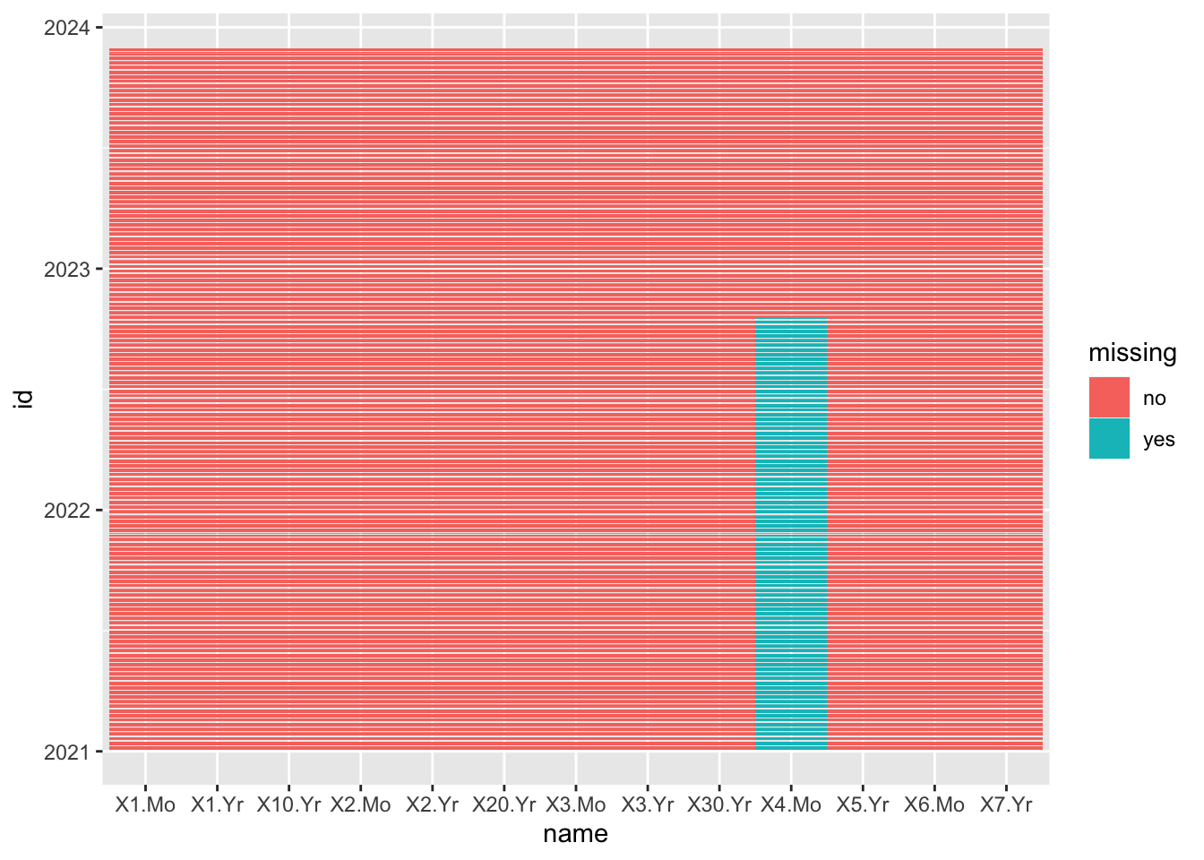

Before 10/18/2022 there are no 4 months interest rates.

Code

start_date <- as.Date("2003-10-29")
end_date <- as.Date("2023-11-05")
date_sequence <- seq(start_date, end_date, by = "1 day")

df <- data.frame(Date = date_sequence)
df$Week_Start_Date <- floor_date(df$Date, unit = "week")
unique_week_start_dates <- unique(df$Week_Start_Date)

template_df <- data.frame(
  Sunday = rep(0, length(unique_week_start_dates)),
  Monday = rep(0, length(unique_week_start_dates)),
  Tuesday = rep(0, length(unique_week_start_dates)),
  Wednesday = rep(0, length(unique_week_start_dates)),
  Thursday = rep(0, length(unique_week_start_dates)),
  Friday = rep(0, length(unique_week_start_dates)),
  Saturday = rep(0, length(unique_week_start_dates))
)

result_df <- cbind.data.frame(Week_Start_Date = unique_week_start_dates, template_df)

result_df <- result_df %>%
  select(Week_Start_Date, Sunday, Monday, Tuesday, Wednesday, Thursday, Friday, Saturday)

Code

sp500_missing <- result_df
sp500_dates <- as.Date(unlist(read.csv("data/GSPC.csv")['Index']))
for (date in sp500_dates) {
    date <- as.Date(date)
    week_start <- floor_date(date, unit = "week")
    day_of_week <- weekdays(date)
    day_of_week <- match(day_of_week, c("Sunday", "Monday", "Tuesday", "Wednesday", "Thursday", "Friday", "Saturday"))
    sp500_missing[sp500_missing$Week_Start_Date == week_start, day_of_week] <- 1
}

Code

meta_missing <- result_df
meta_dates <- as.Date(unlist(read.csv("data/META.csv")['Index']))
for (date in meta_dates) {
    date <- as.Date(date)
    week_start <- floor_date(date, unit = "week")
    day_of_week <- weekdays(date)
    day_of_week <- match(day_of_week, c("Sunday", "Monday", "Tuesday", "Wednesday", "Thursday", "Friday", "Saturday"))
    meta_missing[meta_missing$Week_Start_Date == week_start, day_of_week] <- 1
}

Code

long_df <- pivot_longer(sp500_missing, cols = -Week_Start_Date, names_to = "Day", values_to = "Value")

ggplot(long_df, aes(x = Week_Start_Date, y = Day, fill = factor(Value))) +
  geom_tile() +
  scale_fill_manual(values = c("1" = "cornflowerblue", "0" = "red")) +
  labs(fill = "Value", x = "Week Start Date", y = "Day of the Week", title = "S&P500") +
  coord_flip()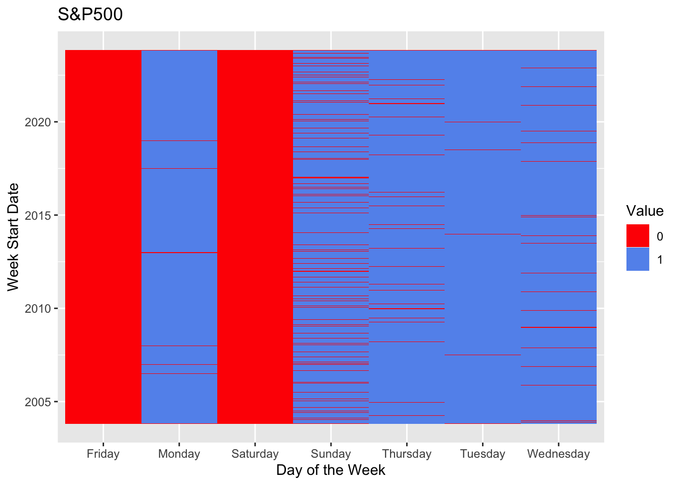

Code

long_df <- pivot_longer(meta_missing, cols = -Week_Start_Date, names_to = "Day", values_to = "Value")

ggplot(long_df, aes(x = Week_Start_Date, y = Day, fill = factor(Value))) +
  geom_tile() +
  scale_fill_manual(values = c("1" = "cornflowerblue", "0" = "red")) +
  labs(fill = "Value", x = "Week Start Date", y = "Day of the Week", title = "META") +
  coord_flip()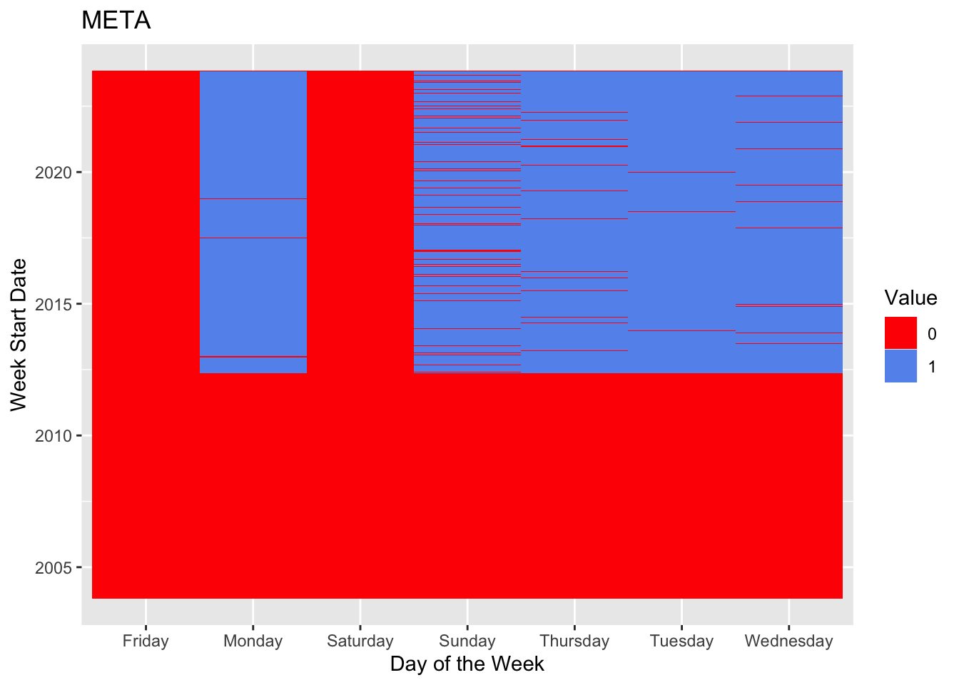

There is no missing value in the stock data. However, due to some stocks entering the market late, earlier data does not exist for those stocks.

While there is no missing data, market closes during holidays, so some dates will miss, but the data from Yahoo is accurate to use.